On the Dynamic Effects of the EU Carbon Border Adjustment Mechanism and Potential Global Responses: An Intertemporal General Equilibrium Exploration (*)

Jean Mercenier

Emeritus Professor of Economics

Université Panthéon-Assas (Paris 2) & CIRED

Ebru Voyvoda

Professor of Economics

Middle East Technical University

A. Erinç Yeldan

Professor of Economics

Kadir Has University

On the Dynamic Effects of the EU Carbon Border Adjustment Mechanism and Potential Global Responses:

An Intertemporal General Equilibrium Exploration

I. Introduction: Statement of the Problem

As indicators of an ecological and climate crisis escalate, pleas for a green transition to attain a net zero emissions global economy by mid-century are increasing. Researchers at the International Panel on Climate Change (IPCC, 2018) assert, for instance, that achieving the 1.5°C objective is feasible; nonetheless, it necessitates “substantial emissions reductions” and “swift, extensive, and unparalleled transformations across all societal dimensions“. The International Energy Agency (IEA, 2023) urges a doubling of the rate of energy efficiency advancements for a green transition and emphasizes the necessity for the implementation of large-scale funding instruments.

Although climate change is indisputably a world-wide concern, its effects are not uniformly dispersed throughout the international economy. Global measures to combat climate change are significantly impeded by the enduring gaps between rich and developing nations regarding ecological, economic, and political challenges.  In the absence of a global authority (a benevolent social planner, as welfare economists would mark it), individual efforts to combat climate change are rendered ineffective. Part of the challenge is due to the so-called free rider problem, where countries, acting along their self-interest unilaterally, tend to rely on others to take action and bear the costs of adjustment, while they contribute little themselves.  All these rest on various forms of the tragedy of commons and the conundrum that environmental protection is ultimately a global public good (Böhringer, et al, 2022).

Nevertheless, the European Union (EU) has recently embarked upon such an initiation and through its Commission announced the instrumentalization of the Carbon Border Adjustment Mechanism (CBAM) so as to align its ambitious climate goals with the patterns of global trade. As part of the European Green Deal and the Fit for 55 Strategy aiming to reduce EU’s greenhouse gaseous emissions by at least 55% by 2030 and achieve a carbon neutral continent by 2050, the CBAM had been inspired to address problems of “carbon leakage” —the displacement of emissions-intensive and trade-exposed (EITE) production to countries with less stringent climate policies— and to safeguard the competitiveness of European industries.

The EU CBAM is announced in late 2019 to initially target a limited range of the so-called EITE sectors, including aluminum, cement, electricity, fertilizers, hydrogen, iron, and steel. It is to be implemented in two phases. In the first phase, importers of the above identified EITE products would be requested to quarterly report the greenhouse gases they emit during their production domestically and abroad. In the second phase, lined up to start in 2026, importers will be required to purchase CBAM certificates reflecting the carbon content of their imports of these goods. The price of these certificates will align with the EU’s Emissions Trading System price, to ensure consistency. Additionally, the mechanism is designed to allow for adjustments if importers can prove that carbon costs have already been incurred in the country of origin so as to avoid double taxation[1].

The rationale and appeal of the CBAM rest on various claims: first is the argument that carbon leakage occurs when firms relocate their production to jurisdictions with weaker environmental regulations, undermining the effectiveness of unilateral climate policies. By imposing a carbon cost on imported goods equivalent to the EU’s domestic carbon price under her Emissions Trading System (ETS), the CBAM is expected to address this challenge. This mechanism is thought to further ensure a level playing field for EU producers along with imported products while incentivizing other countries to adopt stricter climate measures. Second, it allegedly will help reduce unfair import (as well as domestic non-ETS) competition and serve as an intermediary mechanism to ensure competitive neutrality among economies with different pricing schemes over carbon emissions (Böhringer, et al, 2022). Thirdly, by way of its micro incentives over relative prices, it would serve as a corrective device against the persistent subsidies to fossil fuels, coal in particular.  OECD Environment Statistics document that the financial support provided to the suppliers and consumers of the fossil fuels has reached to as much as 1.3 trillion dollars per annum in 2023 (OECD, 2024), reflecting a continued bias in favor of carbon-intensive sources of energy. The CBAM taxation may help eliminate, at least partially, the inefficiencies due to the price distortions emanating from fossil fuel-based input usage.

Finally, the CBAM is thought to reinforce the EU’s role as a global leader in climate action, leveraging its market power to promote decarbonization internationally. Through CBAM, the EU will be able to adopt a viable instrument through which it can reinforce its ETS, aligning domestic and imported carbon pricing within international policy coherence (Gros, 2023; Gros, et al, 2010).

Yet, despite all these theoretical argumentations, the real practices of geopolitical economy responses may as well turn out to be quite different in nature and scope.  First and foremost are the real-world problems due to many unavoidable intricacies of monitoring, verification, and implementation at plant level, within an international spectrum. For one, the CBAM coverage is expected to ultimately expand over embodied indirect emissions, emissions being triggered through carbon-intensive intermediate input demands through the value chain, where proper measurement and monitoring will be prohibitively expensive.

Furthermore, as to be expected the CBAM initiative will have to reckon with the seemingly endless debates on adherence to principles of non-discrimination of the World trade Organization (WTO). EU relies on CBAM’s regulatory characteristics advocating price neutrality, domestic versus border-wise. Many in turn, USA and China in particular, claim that the EU is laying the ground for unfair import protection, while many large export economies of East Asia (which are among the top ten import partners of the EU) reflect that CBAM is inherently a discriminatory policy measure (Böhringer, et al, 2022; Hübner, 2021).

Last but not least, there remain also many unresolved responses, mainly from the global South, underlining the existing –and widening- inequalities of global income distribution and the unabated asymmetries over historical responsibilities of the developed nations in over-exploitation of the global carbon budget –which , according to estimates (as of 2024 ) of the Carbon Independent.org based on IPCC (2018), will run out in seven years in order to keep global warming at 1.5˚C.

Prevailing data indicate that the CBAM sectorial imports constitute only 3% of the aggregate imports of EU.  However, they also appropriate 47% of the free allowances granted to the EU industry. With an estimated CBAM tariff revenue of 7.2 billion euros, they are expected to bring in 15% of tariff burden on aggregate EU imports (Gros, 2023).  In Gros’s remarks, this makes the tax burden of the mechanism to be similar in size, to the various tariffs on steel and aluminum products imposed by Donald Trump during his former presidency.  Thus, at face value the European Union’s carbon border tax can be argued to potentially have only a marginal impact onto the global trade patterns. Yet, acting as a trigger of potential retaliatory responses and strategic re-formation of trade clubs, it could stoke tension among friends (Gros, ibid).  So, it may not be the EU CBAM by itself, but the potential global policy responses that it could potentially trigger, that threaten the patterns of trade and accumulation across the world economy by opening a Pandora’s box of retaliatory measures and club formations.

It is the dual purpose of this article to address these broad concerns, and study not only the isolated trade and welfare effects of the EU CBAM on the global economy, but also to investigate for the arsenal of potential strategic responses of the global trading partners.  We cast the problem within the discipline of general equilibrium, driven by intertemporal dynamics.  Utilizing a multi-regional model, we try to capture the inter-temporal reallocation effects by forward-looking agents under infinite horizon and decentralized inter-temporal optimization. 

Formally, we study four policy scenarios: first, we invigorate the future pathway of the current design of the ETS in EU with a projected cap on ETS sectorial emissions extending to 2050 –the year of carbon neutrality.  Secondly the CBAM is implemented, and its potential macroeconomic and social welfare effects are tabulated.  In what follows we envisage and study two opposing responses from the non-EU global economy: (i) instrumentalization of a retaliation tariff rate across the trade partners, to maintain their individual (regional) social welfare against the EU CBAM; and (ii) a scenario of “cooperation with the EU” via full alignment with the EU_ETS carbon price, accepting the economic rationale of CBAM as a sanctioning instrument (Böhringer, et al, 2022).

The rest of the article is organized three sections. Next, we introduce the salient features of our model, its dimensions, and data sources.  We administer our policy scenarios and provide and analytical discussion in section three; and conclude in section four.

II. Modeling Features and Dimensions

In this section, we provide the main components of the multi-regional general equilibrium model, while the full set of equations are provided in Appendix 1 below. Its analytical structure is based on an extension of Mercenier and Voyvoda (2021) and comprises infinite horizon, decentralized intertemporal optimization dynamics driven by consumption smoothing over time, as well as intra-temporal equilibrium in the commodity and factor markets across both the regional and global economy levels.

The analytical algebraic structure of the model is calibrated to the GTAP 10 and GTAP-E Database (with 2014 serving as the “base year”), where the ensuing equilibrium is interpreted as the long run steady state for the world economy. To ease numerical convergence and stability of the solution algorithm the model is time-aggregated and solved over a restricted set of grid-points on a discrete time axis, t = t₁,t₂,…,T.[2]  Also, as to be discussed further below, the policy of free allowances are known to be phased out by 2034 and our time aggregation scheme respects this schedule by setting the “early” time grids to current calendar dates, while the “later” periods are aggregated across wider time segments.

We partition the world economy under eight regions, where each is designed as an indigenous unit behaving endogenously in response to the given market signals.  Within this aggregation scheme, we maintained the regional entities of EU27, the developed rest of the world (ROW_dvd) and developing rest of the world (ROW_emdc) each as a mono bloc.  In addition, five individual nation-economies are highlighted based on their exposure of exports to the EU to have a sharper focus on the warranted bilateral trade and capital accumulation effects in response to the CBAM scenario and beyond (see Table 1 for details). All regions/countries, as indexed by {i,i’}, are assumed to have identical structures.

Over the production side, the model encompasses 29 sectors, 6 of which are the sectors of renewable and non-renewable electricity production (see Table 1).  Given the sectoral characterizations of the GTAP 10 database, we distinguish the CBAM, EU-ETS and non-ETS sectors as different sectorial units based on the officially set emission targets, direct and indirect emission coverage, and the free allowance calendar as had been announced by the EU Commission. 

All households, in each region are represented by a single representative one that is endowed with labor, which we assume regionally fixed in supply. The labor is allocated, endogenously through a CET allocation frontier, to different sectors, within each region, in response to wage differentials. We control this allocation through an elasticity of transformation parameter. 

Table 1. Dimensions of the Analytical Model

Households are the owners of physical capital, the accumulation of which is dependent on the endogenous saving-consumption decision, based on intertemporal utility maximization. Here, the constant relative risk aversion (CRRA) type period utility function assumption leads to the following necessary condition for optimization:

                                                      (1)

where i is the region and t is the time index.  σ denotes the intertemporal substitution elasticity and ρ is the rate of time preference of the representative household.  represents the t price index of composite consumption good  and is the unit cost of investment at time t.  is the rate of return on private capital as expected in period t, to be reaped at t+1 and is equal to:

                                                               (2)

where   is the unit (rental) price of the physical capital at time t+1. The parameter κ coverts the services of capital into the stock variable. δ is the depreciation rate.

Across the global capital markets a distinguishing feature of the model is its explicit recognition of high mobility for (“financial”) capital. Therefore, in equilibrium there should be no systematic differences among the expected rates of return of capital among the regions, globally. Hence, we have  =  . Additionally, we assume that the capital stock owned by the representative household in each region is pooled into a global capital stock to ensure a homogenous rental price for capital,   that serves for valuation of the physical assets of the households. Yet, we also know that the rental cost of capital varies across regions and across sectors within each region. We capture this feature by allocating the global physical capital to each region/sector pair through a 2-level CET structure. In so doing we attempt capture the complex nature of modern global capital movements where capital ownership at the regional households is not solely restricted to the amount of capital services contributing to the region’s gross domestic product, but represents the international ownership of capital. This feature is especially relevant in addressing the carbon-leakage effects that are expected to emanate both through re-allocation of capital stock and production activities globally. Also, the transformation elasticities are set at dual levels (region, /sector, ) to control the level of concavity of the CET allocation frontiers. Such a structure conveniently depicts the degree of mobility of capital, both inter-regionally and inter-sectorally within each region. The calibration of   and  are naturally linked to the base path steady state equilibrium. Because accumulaiton of the global capital stock also implies the pooling of new investment, we also have   =   .

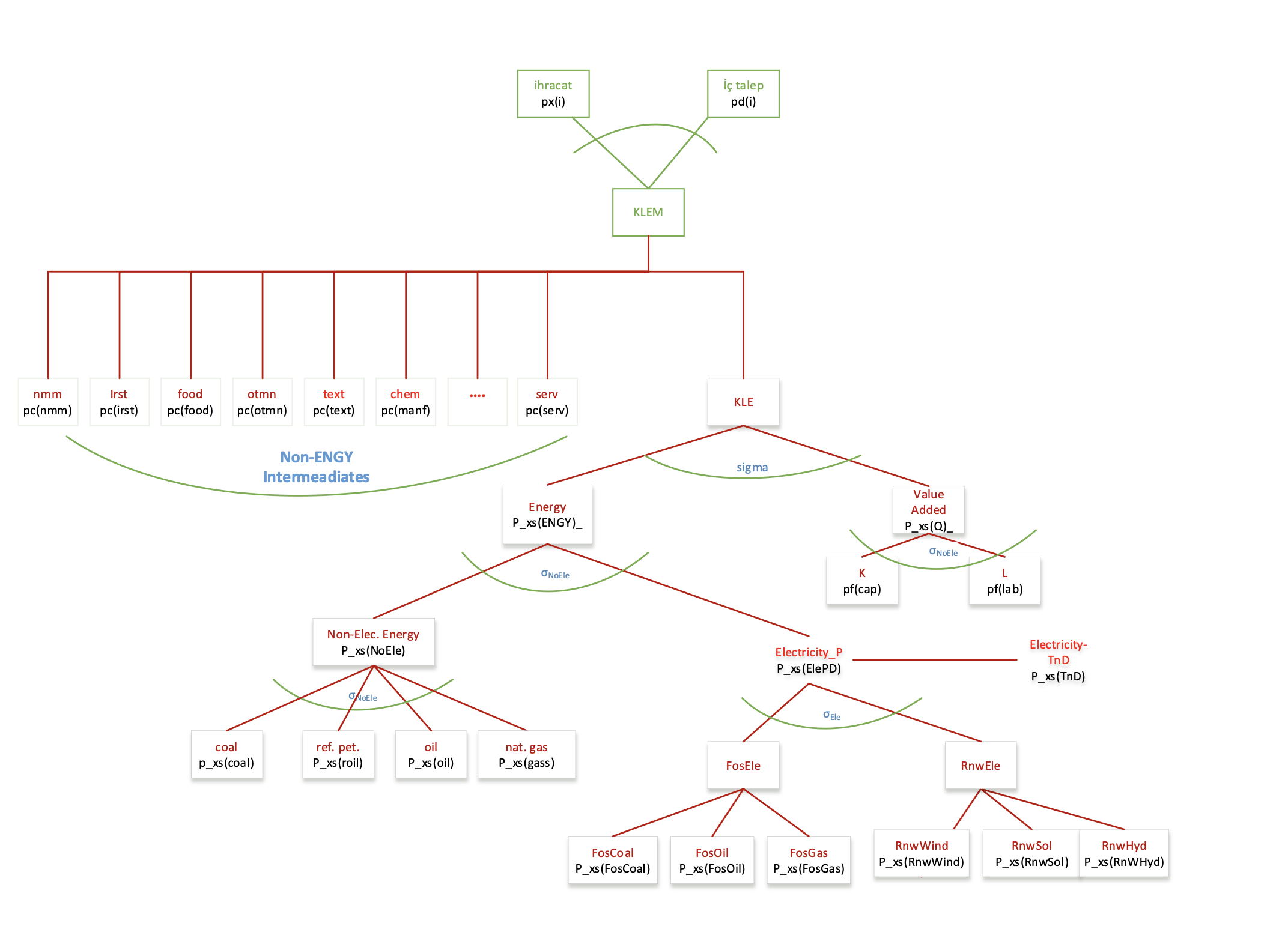
Production activities are narrated via constant returns to scale (CRS) production functions through multi-level nested production structures to produce homogenous (regional) good operating under a perfectly competitive environment. Porduction technology combines energy inputs (primary and secondary), non-energy intermediates, capital and labor through nested structures. The research questions that are investigated in this study naturally demand a detailed representation of (i) primary energy inputs through fossil fuels (ii) electricity production through renewable and non-renewable sources. Therefore, of particular interest is the representation of the nested-CES structures of production.[3] For a representative production sector, the non-electricity primary energy inputs and the secondary electricity input are defined as non-electricity energy (NonEle) and electricity (Ele) composites, associated with elasticity of substitution parameters and  , which then aggregates into a composite energy input. At the upper level, this composite energy input aggregates with material composite and the factors of production embedded in value added, through a further CES substitution elasticity, . Here, aggregate material inputs are also defined as CES bundles of goods from non-energy sectors, through fairly inelastic substitution possibilities.

As CBAM is announced to cover both direct and indirect (scope 1 and scope 2) emissions for fertilizer, electrical energy and cement sectors, we represent both direct (through usage of fossil fuels as primary energy inputs, scope 1) and indirect (through emissions due to electricity input production, scope 2) emissions, in line with the emission coefficient parameters calibrated at the steady state equilibrium. For each sector s, direct emissions dues to primary energy usage becomes:

                                           (3)

where   denotes the (intermediate) input requirement of sector s from sector s’ at time t. For indirect emissions, one has to take into account the electricity demand, , along with the total emissions produced during electricity production.

The public sector in the model serves for calibration purposes mostly and we try to keep the potential macroeconomic impacts of the public sector as neutral as possible through various assumptions. It ought to be noted that such characterization is not a “policy” choice but is mainly instrumentalized to distinguish the social welfare comparability of the scenarios to be implemented.

Each regional aggregate demand,  for each sector’s output comprises of final and intermediate demand and is converted into a trade matrix with non-zero diagonal elements denoting the demand for home goods. Here, we use a CES-allocation structure with inputs  representing demand by region i, the output s produced by region i’ at time t. Under CRS technology, this corresponds to the conventional Armington specification of the AGE folklore.

Finally, the overall model is brought into equilibrium through endogenous adjustments of product and factor prices and the real exchange rate to clear the commodity and labor markets and balance the payment accounts. The EU regional price index serves as the numéraire of the system.

The welfare comparison among scenarios is carried out through the welfare index ψ_i and defined as the equivalent variation (EV):

                                                                  (4)

under the CRRA period utility function based on aggregate consumption. Here, C_i,0 is the initial steady state vale of aggregate consumption in region i. Ψ_i is the discount factor for households in region i.

The calibration of the model,  naturally depends on the initial choice of the parameter set, which we present in Appendix Table A2. We run a set of sensitivity analyses for a set of parameters and report the comparative results in Appendix 2.

III. Policy Analysis

III-1. The ETS Pathway

The EU has introduced the ETS as the main instrument to control emissions in 2005. It now covers greenhouse gas emissions from around 10,000 installations in the energy sector and manufacturing industry, as well as aircraft operators. From 2024 onwards, the EU ETS also covers emissions from maritime transport.

Due to the excessive surplus created by free allowances in the first years of operation of the system, the carbon market failed to generate “positive” prices. The “market” started to function after 2013, when the constraints on the allocations became binding.  The EU ETS is currently in its fourth phase, which extends from 2021 to 2030. Throughout this period, auctioning continues to be the principal technique for allocating allowances. The overall emissions cap has been set to be reduced each year by a linear reduction factor, set to 4.3% yearly from 2024 to 2027, then to 4.4% annually from 2028, targeting a 62% reduction in emissions by 2030 relative to 2005 levels.

The ETS trajectory is further driven by the projected calendar on phasing out the free allowances, where following the 2023 revision of the ETS Directive, the EU has planned to start reductions in 2026 to be completed by 2034. To prevent leakage, the ETS has been allocating free allowances to the sectors with higher risks of carbon leakage such as chemicals, cement and lime, iron and steel, and mineral oils.  These allowances permit companies to emit a specified amount of greenhouse gases without purchasing additional permits, where each allowance permits the emission of one ton of CO₂ equivalent.

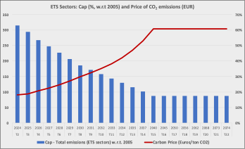
In what follows, we implement the ETS cap as specified under the official rates indicated above.  Beyond 2040, it is assumed that the cap will remain constant at 18% (against the 2005 levels –the initiation of ETS). The resulting traded value of the EU Allowances (EUAs) –carbon price- is to be determined endogenously by the model.

Model’s solutions on the trajectory of the ETS quota with due adjustments of phasing out of the free allowances being imposed are depicted in Figure 1.  The carbon price, which was on the order of 85 euros at the time of writing, is projected to rise to 300 euros by 2040 and stabilizes then after as the cap is set constant at 18%.

Figure 1. Pricing Carbon under the ETS Quota Trajectory

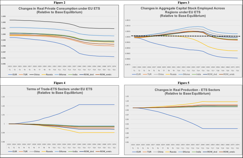
The unilateral pricing of carbon within the EU geography under such a steep trajectory induces a series of adjustments both at home (among regions) and abroad.  We display the adjustment paths of the most relevant macroeconomic variables under Figures 2 through 5.  As to be expected, EU decelerates as costs of production effectively are bid up due to pricing carbon. EU ETS sectors shrink by as much as 9% in real terms towards the long run equilibrium. Looking at private household welfare EU households’ losses are observed to be on the order of 0.02% per annum in the short run, to deepen up to 0.2% in the medium to long run (relative to base equilibrium), with a permanent decline stabilizing after 2040. Likewise, increased costs in EU reduce profitability; thus, the share of EU in global capital allocation diminishes (as disclosed in Figure 3).  Deceleration of the economic activities in Europe pulls its significant trade partners along and Russia, Türkiye and India follow the EU’s tjectoryra even though at a modest rate.  China and South Korea, along with a lesser extent and in the short run, the Developed ROW, stand to gain as the EU takes the brunt of environmental abatement.

The regional terms of trade carry on the relative price signals across the global markets.  Induced by the carbon costs, the ETS sectors in EU suffer from relative price rises by 0.6% by 2030 to stabilize at around 2.1% under the new long run equilibrium.  Russia, being a significant net exported of mostly natural gas and oil as key intermediates with low elasticities of demand, suffer from the contraction of demand from EU with a fall in its terms of trade in the ETS sectors identified (Figure 5).

Figures 2-5: Intertemporal Adjustments of Selected Macro Indicators under ETS (Changes Relative to Base Equilibrium)

III-1-1. Carbon Leakage Revisited

As the above discussed macro adjustments occur, we can read the ensuing repercussions in global gaseous emissions.  Commensurate with the decline of economic activity in the EU, its emissions are observed to recede; and yet to be re-generated elsewhere in the non-EU global economy due to favorable relative cost margins.  Thus, carbon emitted within the EU ETS is expected to leak through economic expansion elsewhere.  This (carbon) leakage is observed to be the outcome of three major effects within the context of our analytical model: (i) Competitiveness Channel, through which carbon pricing under emissions trading increases production costs for firms in regulated jurisdictions. This will incentivize (fossil fuel-intensive) production and physical capital to be relocated to regions with less stringent climate policies; (ii) Intermediate Fossil Fuel Market Channel, through which reductions in  fossil fuel demand within the regulated ETS product markets can lead to lower prices. Relatively cheapened fossil fuels may then stimulate increased consumption in the unregulated non-ETS product markets; and finally (iii) Trade Channel where importing goods from countries with lax emission controls replaces domestically produced goods under stringent carbon policies (see, Felder and Rutherford, 1993; Burniaux and Oliveira-Martins, 2012; and Böhringer, et al, 2022 for original statement and further discussion of the problem).

Böhringer et al (2022) and Böhringer et al (2012), based on their reviews of CGE analyses, report that central estimates of carbon leakage range between 5% to 30% for the industrialized economies. In contrast, Branger et al, 2016; Healy et al, 2018; Naegele and Zaklan, 2019; Venmans et al, 2020 studied the leakage rates in the EITE sectors of the EU ETS, and reported estimates with low significance statistically.  In any case, carbon leakage is not expected to be homogeneous throughout the economy with high-energy sectors exposed to trade, such as cement, steel, and aluminum, showing considerable higher leakage rates (Mehling, et al, 2019), and a more focused calculation at the sectorial level is warranted.

Given our general equilibrium results, we carry this exercise and calculate the rate of carbon leakage (to the non-EU global economy, from the EU) in response to the ETS policy environment, as the ratio of the change in CO2 emissions in Region R (R EU) in comparison to the change in emissions in EU.  Thus;

                                              (4)

Results are tabulated in Table 2.

Table 2. Estimates of Carbon Leakage under EU ETS Pathway

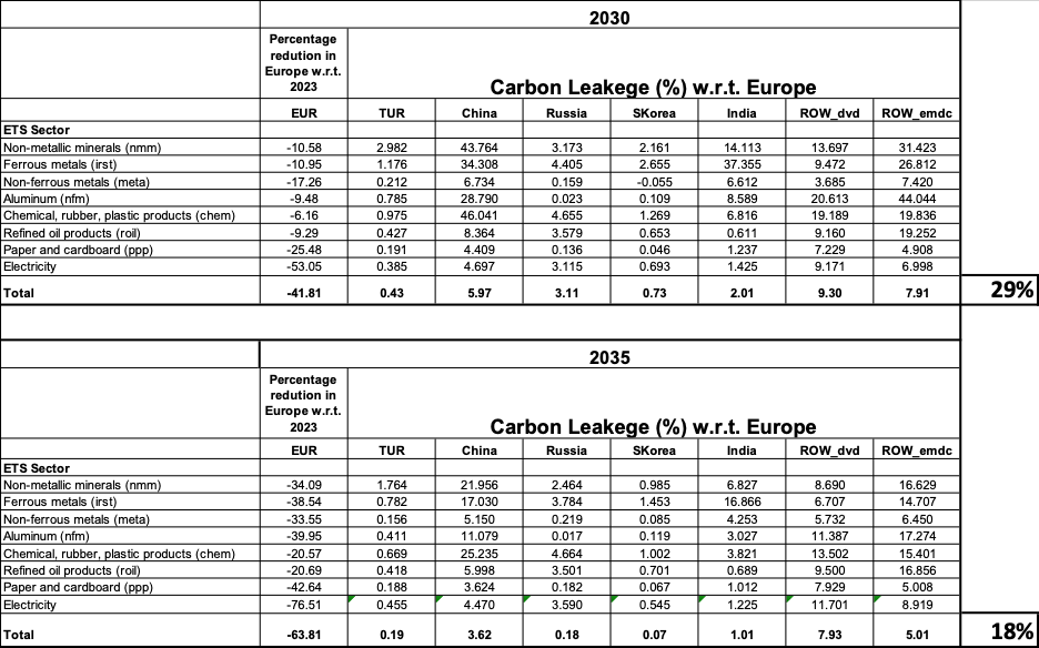
Source: Authors’ calculations based on modeling results.

Our results suggest that by 2030 reduction in carbon emissions from the ETS sectors stand at 41.8% (with respect to 2023 levels).  Through the intertemporal general equilibrium channels described above, 29% of this reduction leaks out –that is, global emissions could be reduced, net, only by two thirds of the 41.8% in 2030.  By 2035 reduction of emissions reach to 63.8% in EU, and yet 18% of it continues to leak out to the non-EU global economy.

At the regional level, it is observed that by 2030 the developed economies disclose the major share of leakage with a rate of 9.30%).  Emerging/developing countries and China follow with rates 7.91% and 5.97%, respectively.  Türkiye (0.43%) and S. Korea (0.77%) have relatively low shares of the leakage; and Russia and India display moderately high responsibilities with rates of 3.11% and 2.01%, respectively.

III-2. Implementation of CBAM by the EU

EU reacts by way of initiation of carbon border tariffication (CBAM) in the flowing five sectors: cement, iron-steel, aluminum, electricity, and fertilizers.

According to the proposal adopted by the European Parliament (European Parliament, 2022), the 2023-2026 period is determined as a pilot phase during which only 5 products, cement, iron-steel, aluminum, electricity, and fertilizer will be covered.  In the meantime, a new EU-wide central CBAM authority will be formed to administer the process.  EU importers of these products are required to register to this authority and report and have the Scope 1 (direct) emissions embedded in the imported products verified to an independent agency that is also required to be accredited by the CBAM authority.  During the pilot phase, EU importers are only required to report the emissions. The payments will start by 2027.

Accordingly, for each ton of green-house gaseous emissions, EU importers ought to buy one unit of CBAM Certificate. The price of the CBAM Certificate will be the average price under the EU ETS during the relevant week.  Along this calendar of events, the tax burden of the CBAM on the EU importers will need to be adjusted given the plans to phase out the remaining free allowances. Since free allocation under the EU ETS has been decided to continue until 2034 (with gradual reduction starting by 2027), the same policy will be applied to the non-EU producers of relevant products (determined as carbon-leakage risky under the EU ETS).

Finally, to avoid double taxation, the carbon price paid at the origin country will be deducted from the price to be paid at the EU border, and the revenues generated by the selling of CBAM Certificates will be channeled into the EU Budget and will not be returned to the originating country as opposed to the implementation under the EU ETS.

The limited product and emission coverage are subjects of discussion among the decision makers in the EU. The EU Parliament recently proposed to include more products such as organic chemicals, plastic polymers, hydrogen, and ammoniac to the list and to extend emission coverage to include Scope 2 as well.

Formally we implement the CBAM scenario where the carbon border tariff revenues are calculated by the emission intensity times the difference of carbon price in EU versus Region R (mostly zero) times exports from region R to EU:

                        (5)

where the first term on the right gives the carbon intensity (CO2_i / Q_i) for the identified CBAM sectors above; and the term in the parentheses is the carbon price differential between the EU and that of the exporting region R; with the export magnitude, E_i, given by the last term on the right.  Dividing the aggregate tariff revenues by the realized import bill yields the CBAM tariff rate.

Given that ETS is a historical reality by now, we report our results relative to the ETS equilibrium solved under scenario ETS above.  Thus, the results of the CBAM will directly allow us to measure the effectiveness of the expected intertemporal adjustments against the EU’s legislative proposed.  We display the relevant adjustments in Figures 6 – 11.

Under the CBAM intervention, relative to the ETS equilibrium, EU stands to gain in terms of private household welfare upon impact and in the short to medium time horizon.  Private consumption is observed to be on a rising pathway in real terms till 2030, then to be adjusted downwards under intertemporal optimization (Figure 6).  As the added tariff burden on CBAM imports is known to materialize more effectively beyond 2030, EU households adjust by intertemporally moving their consumption expenditures to short run and switch to a higher savings pathway after 2030.  This behavior leads to a rate of higher capital stock formation in the EU after 2030s (Figure 7), while the rest of the global economy suffer from lower capital accumulation rates under the long run equilibrium.

As the most export-dependent economy to EU for the CBAM sectorial intermediates, Russia suffers from the CBAM tariffication, and its real private consumption permanently declines as measured against the ETS pathway. India and China as well disclose declines in private consumption, albeit in quite modest rates, while Türkiye along with the developed and developing regions of the world economy do not seem to be significantly affected. 

Terms of trade experienced by the ETS sectors serve as the main triggering mechanism of these adjustments (Figure 8), with increased tariffs in the EU CBAM sectors leading to increased prices.  Decline in import demand from the EU leads to significant falls in China, Russia, Türkiye and India due to their relatively high exports shares for Europe.  CBAM sectorial exports to Europe fall by 38% in 2030 in India, where it settles with a loss of 80% under the new long run, steady state equilibrium.  By 2030, CBAM exports to EU are observed to fall by 18% in China and Russia; 13% in Türkiye; and by 14% and 5.6% in the developing and the developed economies of the world economy (Figure 10).

Figures 6-11: Intertemporal Adjustments of Selected Macro Indicators under CBAM (Changes Relative to ETS Equilibrium)

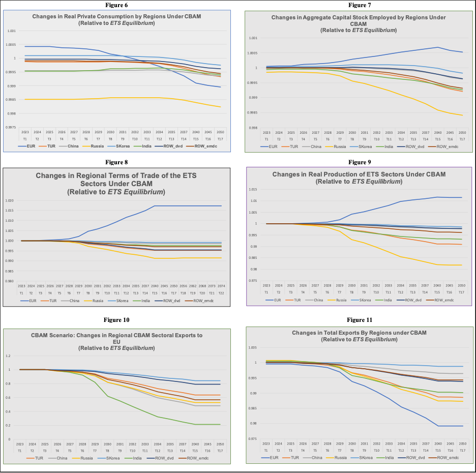
The effects of these variations on the aggregate regional exports depend upon the overall share of the CBAM sectors in the totals, as well as on the observed intensities of the CBAM emissions across regions in the first place. Russia, Türkiye and India, disclosing relatively high emission intensities and export shares of the CBAM sectorial aggregate and significantly suffer comparably deeper declines in their total exports (Figure11).  S Korea, due to its relatively low export share and low emission intensity, is observed to be minimally affected from the CBAM scenario of events.

All considered, the CBAM sectorial production activity settles at a lower plateau in the long run with permanent real output losses of 1.75% in Russia; 1% in Türkiye; and close to 0.5% in India and the developing economies (See Figure 9, all relative to the ETS equilibrium).

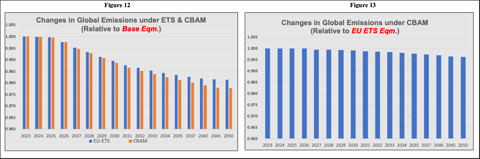
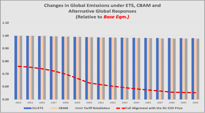
If we were to take stock of what the post-ETS and post-CBAM policy interventions would bring to the global emissions as a whole, the model results reveal relatively very modest gains if at all.  In Figure 12 we disclose the pathway of global emissions under the ETS imitative of the EU.  As to be observed, the model results suggest that relative to the base path equilibrium, mitigation attempts via the unilateral implementation of a carbon pricing scheme in Europe within the selected ETS sectors has a very low impact.  Compared to base pathway, gains in gaseous emissions reach only to 1.1% by 2035, when the phasing out of free allowances in the ETS is completed, and to 1.9% at the end of the net zero transition, 2050.  This is depicted in Figure 12, while Figure 13 discloses the gains in total emissions upon the initiation of the CBAM tariff protection in the EU against the ETS equilibrium.

Our findings reveal that, compared to the ETS, with the initiation of the CBAM –to allegedly combat the threat of carbon leakage, changes in global emissions stand only on the order of 0.1% in 2030, to permanently settle down to 0.3% by 2050. 

Figures 12 & 13: Changes in Global Emissions under the ETS and CBAM pathways

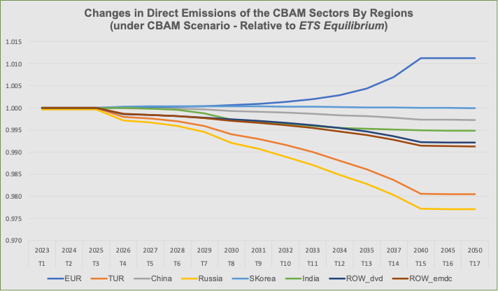
To complete these assessments, we also display the regional direct emissions of the CBAM sectors in Figure 14.  We find that Russia and Türkiye contribute the most to the global reduction of emissions, with mitigation rates of 0.8% and 0.6% by 2030; and 2.3% and 2.1% by 2050, respectively.  China’s and India’s reduction rates are more modest, with 0.3% and 0.5% in 2050; and the developing ROW by 0.9%.  S. Korea remains almost neutral in mitigation. 

It is critical to note that the EU ends up increasing its emissions along the CBAM sectors that it purported to control against leakages.  Compared with the ETS pathway, EU’s CBAM sectoral emissions rise by 0.1% in 2030; and by 1.1% 2050, negating a sizable portion of the gains under ETS.  This is due to the tariff protection advanced over these sectors and the very fact that CBAM sectorial activity does get invigorated at the end of the day (see Figure 9 above).

Figure 14: Changes in Regional Direct Emissions of CBAM Sectors under the CBAM Equilibrium (Relative to ETS Equilibrium)

The dismal nature of these findings rests on the fact that the ETS sectors cover roughly at most half of Europe’s total emissions, where the latter constitute a meager 6.4% of the global total.  Thereby, the EU initiative falls too short, too late in generating a global dent in the emissions dynamics.  There also remain institutional shortcomings.  In its evaluation of the Future of the Emissions Trading in the EU, ERCST (2024) notes, for instance, that “the EU ETS did not and does not provide a full price signal”.  The ERCST report further remarks that, “a full price signal coupled with effective carbon leakage risk mitigation is important to trigger low carbon investments and to incentivise a changing behaviour aligned with net zero goals”.

Notwithstanding, both the ETS and the upcoming CBAM remain strongholds in current climate policy agenda, with an array of potential responsive strategies in the making. It is to this subject we now turn our attention.

III-3. Studying Potential Global Responses against CBAM

In what follows, we administer two divergent pathways of global response against the CBAM: at one end, the CBAM and its aftermath may trigger a set of retaliatory trade measures among the non-EU nations, leading to a rise of global sentiment towards trade protection.  On the other, one can also conjecture a global understanding of full alignment with the EU carbon pricing policies, thereby accepting its initiative (as already self-advocated by the EU within a non-revealed diplomatic stance).

The first counter-scenario designs the retaliation of tariffs response in two steps:

• each country (region) individually decides in a myopicmanner on its retaliation tariff in partial equilibrium, each one at a time, to compansate for the loss of its national (regional) social welfare under the CBAM
• all countries (regions) simultaneously implement their individual tariffs as planned in (1) above.

Technically speaking, the tariff retaliation scenario seeks for the results of a once-and-for-all, von Stackelberg game with no coordination.  Under the other extreme we envisage that the non-EU countries agree upon fully aligning with the EU’s ETS carbon price to be implemented in their own jurisdictions.  Thus, we set

                                                      (7)

with the consequent result that, the CBAM tariff rate collapses to nil (equation 5). 

Amidst absence of a global social leader capable of imposing an optimal global carbon price, the scenario mimics a loosely articulated “cooperation” scenario.  The EU long advocates that her initiatives to combat emissions via a system of carbon trading that make use of market pricing instruments as much as possible, is the most efficient way towards the net zero pathway.  The design rests its theoretical bases on the in seminal discussions put forward in, e.g., Helm, et al, (2012), Al Khourdajie and Finus (2020), and Lessmann, et al (2009), establishes a  non-coordinated sanctioning instrument, which, in the words of Böhringer, et al, (2022), could act as a game changer combining trade sanctions with a climate club acting for the global public interest for the benefit of all.

We start the tariff retaliation scenario by first reporting on the changes in aggregate private household welfare realized under implementation of the CBAM by the EU.  Table 3 displays the findings relative to the ETS equilibrium.

Table 3. Estimated Changes (%) in Aggregate Private Household Welfare under CBAM

(Relative to ETS Equilibrium)

Given the private household welfare losses over the ETS affairs, each country now is set to decide on a tariff rate that will suffice to compensate those losses.  The tariff is to be imposed on the respective CBAM sectorial imports from the EU.  Technically speaking, we rely on the laboratory characteristics of our general equilibrium model and endogenously solve for the rate of tariff to be imposed on the CBAM imports, given the household welfare “level” along the intertemporal ETS pathway.  To further neutralize the fiscal effects of the tariff revenues, we constrain the real level of fiscal revenues to the ETS pathway and create an endogenous tax/subsidy scheme that adjusts continuously to leave the fiscal revenues unabated to the tariff revenues generated.  Thus, the model results of the scenario are abstained form any macroeconomic effects emanating from the fiscal operations of the governments and are dependent solely on the trade effects of tariffication responses.

The resultant pathways for the regional tariff rates are displayed in Figure 15.  It ought to be underlined that the resolution of the retaliatory tariff pathway is subject to complicated intertemporal general equilibrium effects that we can only comment on numerically.  With the accommodation of the theoretical hypothesis of perfect foresight under an infinite horizon framework, private households invigorate their optimal plans to smooth out their consumption trajectories in response the declaration of CBAM tariffs. 

Figure 15

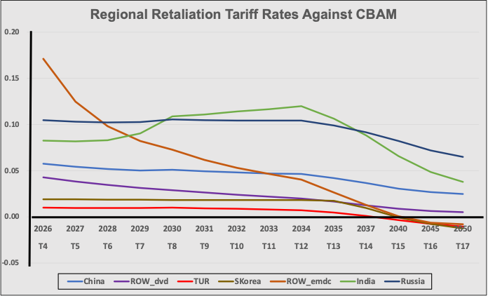
We observe that the most vivid reaction comes from the Developing ROW with a tariff rate of 17% upon impact (in 2026, with the advocation of the CBAM profile). Russia initiates its tariff at 11%, India at 8% and China at 5%.  It is interesting to note that S Korea is set to implement a higher rate of tariffication compared to Türkiye, and that both countries choose a negative tariff rate (subsidy on CBAM imports) after the 2040s. 

In fact with the proviso of the discount rates imposed across households’ consumption profile, tariff adjustments are more pronounced upon impact and in the short run, to be smoothed out and alleviated towards the very long run.

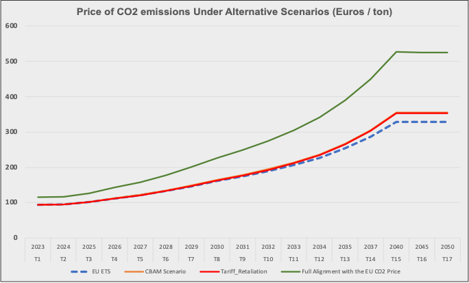
Figure 16 spells out the carbon price under the two global responses.  We read that tariff retaliation has very little effect, if any, on the ETS equilibrium price, while the scenario of “Full Alignment” leads to a very significant and steep increase of the carbon price to reach higher than 500 euros by 2040.  Clearly as the EU sets course to maintain its cap on the ETS sectors, and the non-EU economies follow suit, the signaling effects become amplified all through the global economy as the price advantages are neutralized across.  With the burden of adjustment falling solely on the EU ETS sectors to sustain the initial cap on their respective emissions, the carbon price is bid up upwards.

Figure 16

The end result is a significant gain in the global emissions under the full alignment pathway.  As Figure 17 portrays, relative to the base path, global emissions are set to be reduced by 25% upon impact and by 45% by 2050.  In contrast, emissions mitigation is fairly small under the tariff retaliation equilibrium, underlying the power of an effectively designed carbon price scheme.

Figure 17

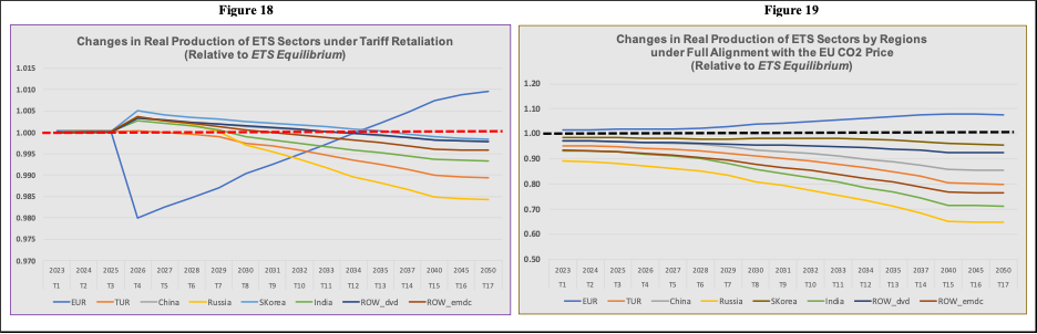
The burden of adjustments is to be followed from the ETS sectors.  Summarized in Figures 18 and 19, we find that tariff retaliation hurts the EU ETS sectors the most, as to be expected. Yet, what is informative to read is that along the intertemporal adjustments due following the 2030s, the non-EU global economy starts to falter as the cost of efficiency losses sink in.  Deceleration of the non-EU regions work to relative advantage of the EU, and the ETS sectors stand to gain under steady state equilibrium. This effect is more visible in Figure 19 which narrates the set of adjustments foreseen by the EU ETS against when all the non-EU regions face the same burden of carbon pricing and relatively stand in a more advantageous position (Figure 19).

Figures 18 & 19: Changes in Real Production of the ETS Sectors under Alternative Global Responses

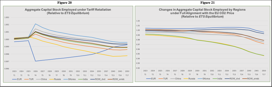
Intertemporal consumption smoothing call for a rapid substitution of consumption expenditures towards the current periods in the EU. In contrast, coupled with relatively higher prices in the ETS global markets, the non-EU producers find it more profitable to increase capital investments and generate higher pathways (Figure 20), Russia being the single most exception. Capital stock accumulation follows a more neutral course under Full Alignment scenario; nevertheless, Russia and India are observed to sustain significant departures from the other regions of the global economy (Figure 21).

Figures 20 & 21: Changes in Regional Aggregate Capital Stocks under Alternative Global Responses

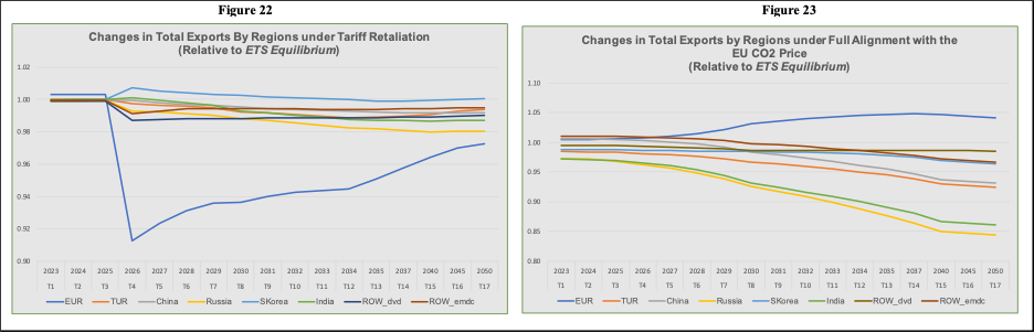
When it comes to the global trade patterns, the general result is that tariff retaliation leads to a significant downward adjustment in the EU aggregate exports –by 8.4% upon adjustment (Figure 22) to be contrasted by their slow but steady rise under the Full Alignment response (Figure 23).   Full Alignment scenario reveals a contracting trade environment for the global economy at large, with Russia, India and to a lesser extent Türkiye suffering the most declines.

Figures 22 & 23: Changes in Regional Aggregate Exports under Alternative Global Responses

Finally, we take stock of the (private household) welfare consequences.  Bringing all three scenarios together –the CBAM, tariff retaliation, and full alignment with the EU carbon price, we observe that the overall re-adjustment of welfare is significantly positive for Europe under Full Alignment, in contrast to modest (CBAM) to not-so-modest (tariff retaliation) scenarios. Perhaps the most important result to be noted here is the finding that under CBAM pathway, the EU households do stand to lose welfare as well.  As Table 4 summarizes, China and Russia have small, yet positive, welfare gains under tariff retaliation, but they end up being the most severely hit economies under full alignment equilibrium.  S. Korea, in turn gains significantly after the full alignment scenario, with almost no effect faced under tariff retaliation.

Table 4.

IV. Conclusions and Policy Lessons

In this paper, utilizing a multi-region intertemporal general equilibrium model, we studied the potential effects of the EU’s recent climate-cum-trade policy initiative of the Carbon Border Adjustment Mechanism (CBAM).  The EU CBAM was announced in late 2019 to initially target a limited range of the so-called emissions-intensive and trade-exposed (EITE) sectors, including aluminum, cement, electricity, fertilizers, hydrogen, iron, and steel.  Following the current period of solely reporting, CBAM is slated to become effective in 2026.  As part of the European Green Deal and the Fit for 55 Strategy aiming to reduce EU’s greenhouse gaseous emissions by at least 55% by 2030 and achieve a carbon neutral continent by 2050, the EU rests its CBAM strategy on the arguments of combating potential carbon leakage and safeguarding the competitiveness of its industries as it purports to align its ambitious climate goals with the patterns of global trade. 

We start our analysis by first implementing the EU’s ETS, which is currently in its fourth phase, extending from 2021 to 2030. Accordingly, the overall emissions cap will decrease each year by a linear reduction factor, targeting a 62% reduction in emissions by 2030 relative to 2005 levels. Adopting this official linear reduction timeline along with the projected calendar on phasing out of the free allowances, to be completed by 2034, we project a market-clearing price for carbon under the ETS realm reaching to 350 euros per ton and stabilizing then after under the net zero targets.

Our findings reveal that in response to unliteral pricing of carbon along its ETS, the EU ETS sectors decelerate and shrink by as much as 9% in real terms as costs of production effectively are bid up. As for private household welfare, EU households’ losses are observed to be on the order of 0.2% in the medium to long run (relative to base equilibrium). Likewise, increased costs in EU reduces profitability and the share of EU in global capital allocation diminishes, pulling along its major trading partners, Russia, Türkiye and India, though at a modest rate.  China and South Korea, along with a lesser extent and in the short run, the developed rest of the world stand to gain as the EU takes the brunt of environmental abatement.

Given the general equilibrium adjustments based on inter-temporal optimization, we calculate the rate of carbon leakage (to the non-EU global economy, from the EU), as the ratio of the change in CO2 emissions in Region R (R EU) in comparison to the change in emissions in EU, after the introduction of the ETS Scenario.

Our results suggest that by 2030 reduction in carbon emissions from the ETS sectors stand at 41.8%, reaching to 63.8% by 2035 (both with respect to 2023 levels).  We calculate that 29% of the reduction in 2030 leaks out, that is global emissions could be reduced, net, only by two thirds of the 41.8% in 2030.  The leakage rate is calculated to be 18% by 2035.  At the regional level, it is observed that by 2030 the developed economies disclose the major share of leakage with a rate of 9.30%.  Emerging/developing countries and China follow with rates 7.91% and 5.97%, respectively.  Türkiye (0.43%) and S. Korea (0.77%) have relatively low shares of the leakage; and Russia and India display moderately high responsibilities with rates of 3.11% and 2.01%, respectively.

References

Al Khourdajie, A. and M. Finus (2020) “International environmental agreements and carbon border adjustments” European Economic Review, 124: 102405.

Branger, Frederic, Philippe Quirion and Julien Chevallier (2016) “Carbon Leakage and Competitiveness of Cement and Steel Industries Under the EU ETS: Much Ado About Nothing”, The Energy Journal, 37: 109-135

Boocker, S. and D. Wessel (2024) “What is a Carbon Border Adjustment Mechanism?” Brookings Commentary, July.

https://www.brookings.edu/articles/what-is-a-carbon-border-adjustment-mechanism

Böhringer, C., C. Fischer, K. E. Rosenfahl & T. Rutherford (2022) “Potential Impacts and Challenges of Border Carbon Adjustments” Nature Climate Change 12 (Jan): 22-29.

Böhringer, C., J. Schneider. & E. Asane-Otoo (2021) “Trade in Carbon and Carbon Tariffs” Environmental & Resource Economics 78: 669–708

Böhringer C, Balistreri EJ and Rutherford TF (2012). The role of border carbon adjustment in unilateral climate policy: Overview of an Energy Modeling Forum study (EMF 29). Energy Economics, (34): S97–S110.

Burniaux, J. M. and J. & Oliveira-Martins “Carbon leakages: a general equilibrium view”,  Economic Theory 49: 473–495 (2012).

Carbon Budget (2024) The global CO2 budget runs out in 7 years:

https://www.carbonindependent.org/54.html

ERCST (European Roundtable on Climate Change and Sustainable Transition) (2024) Future of emissions trading in the EU: Role of Emissions Trading in EU Climate Policy, (With lead authors: Andrei Marcu, Juan Fernando López Hernández, Alexandra Maratou, Pauline Nouallet, and Nigel Caruana)

https://ercst.org/future-of-emissions-trading-in-the-eu-role-of-emissions-trading-in-eu-climate-policy/

European Commission (2019) The European Green Deal”, Brussels.

European Commission (2021a) Proposal for a Regulation of the European Parliament and of the Council Establishing a Carbon Border Adjustment Mechanism, Brussels

https://eur-lex.europa.eu/legal-content/EN/TXT/?uri=celex:52021PC0564

European Commission (2021b) Carbon Border Adjustment Mechanism: questions and Answers, Brussels. https://ec.europa.eu/commission/presscorner/detail/en/qanda_21_3661

Felder, S. & Rutherford, T. F. (1993) “Unilateral CO2 reductions and carbon leakage: the consequences of international trade in oil and basic materials”, J. of Environmental Economics & Management 25: 162–176.

Gros, Daniel (2023) The Economic Case for Europe’s Carbon Border Tax, Project Syndicate, October.

https://www.project-syndicate.org/commentary/eu-economic-rationale-for-carbon-border-adjustment-mechanism-trade-tension-by-daniel-gros-2023-10

Gros, Daniel, Egenhofer, Christian, Fujiwara, Noriko, Guerin, Selen Sarisoy and Georgiev, Anton (2010) Climate Change and Trade: Taxing Carbon at the Border? CEPS Paperbacks.  https://ssrn.com/abstract=1618297

Healy, S., Schumacher, K. & W. Eichhammer (2018) “Analysis of carbon leakage under Phase III of the EU Emissions Trading System: trading patterns in the cement and aluminum sectors”. Energies 11: 1231.

Helm, D., Hepburn, C. and G. Ruta (2012) “Trade, climate change, and the political game theory of border carbon adjustments”, Oxford Review of Economic Policy (2): 368–394.

Hübner, C. (2021) Perception of the Planned EU Carbon Border Adjustment Mechanism in Asia Pacific — An Expert Survey, Konrad-Adenauer-Stiftung.

https://www.kas.de/en/web/recap/single-title/-/content/perception-of-the-planned-eu-carbon-border-adjustment-mechanism-in-asia-pacific-an-expert-survey

Intergovernmental Panel on Climate Change (IPCC) (2018) Global Warming of 1.5⁰C. https://www.ipcc.ch/sr15/

International Energy Agency (IEA) (2023) World Energy Outlook 2023, Paris.

https://www.iea.org/reports/world-energy-outlook-2023

Kun Zhang, Yun-Fei Yao, Xiang-Yan Qian, Yu-Fei Zhang, Qiao-Mei Liang, Yi-Ming Wei (2024) “Could the EU carbon border adjustment mechanism promote climate mitigation? An economy wide analysis”, Advances in Climate Change Research, 15(3): 557-571.

Lessmann, K., R. Marschinski, and O. Edenhofer (2009) “The effects of tariffs on coalition formation in a dynamic global warming game”, Economic Modeling, (26): 641–649.

Mehling M A, Asselt H van, Das K, Droege S and Verkuijl C (2019) “Designing Border Carbon Adjustments for Enhanced Climate Action” American Journal of International Law, 113(3): 433–481,

Naegele, H. & A. Zaklan (2019) “Does the EU ETS cause carbon leakage in European manufacturing?” J. of Environmental Economics & Management 93: 125–147.

OECD (2024) OECD Inventory of Support Measures for Fossil Fuels 2024: Policy Trends up to 2023, OECD Publishing, Paris. https://doi.org/10.1787/a2f063fe-en.

Venmans, F., Ellis, J. & D. Nachtigall (2020) “Carbon pricing and competitiveness: are they at odds?” Climate Policy, 20: 1070–1091.

---

[1] For official announcement of the CBAM and related material, see European Commission (2019; 2021a; 2021b); for a descriptive summary for the general audience, see Boocker and Wessel (2024).

[2] See Mercenier and Michl (1994) for further details on time aggregation issues in intertemporal models.

[3] Figure A1 in the Appendix shows an illustration of the nested-CES structure of production for a representative sector, long with the associated CES parameters at each stage.